11. NumPy
“Let’s be clear: the work of science has nothing whatever to do with consensus. Consensus is the business of politics. Science, on the contrary, requires only one investigator who happens to be right, which means that he or she has results that are verifiable by reference to the real world. In science consensus is irrelevant. What is relevant is reproducible results.” -- Michael Crichton
11.1Overview
NumPy is a first-rate library for numerical programming
- Widely used in academia, finance and industry.
- Mature, fast, stable and under continuous development.
We have already seen some code involving NumPy in the preceding lectures.
In this lecture, we will start a more systematic discussion of
- NumPy arrays and
- the fundamental array processing operations provided by NumPy.
(For an alternative reference, see the official NumPy documentation.)
We will use the following imports.
import numpy as np
import random
import quantecon as qe
import matplotlib.pyplot as plt
from mpl_toolkits.mplot3d.axes3d import Axes3D
from matplotlib import cm11.2NumPy Arrays
The essential problem that NumPy solves is fast array processing.
The most important structure that NumPy defines is an array data type, formally called a numpy.ndarray.
NumPy arrays power a very large proportion of the scientific Python ecosystem.
To create a NumPy array containing only zeros we use np.zeros
a = np.zeros(3)
a
array([0., 0., 0.])type(a)numpy.ndarrayNumPy arrays are somewhat like native Python lists, except that
- Data must be homogeneous (all elements of the same type).
- These types must be one of the data types (
dtypes) provided by NumPy.
The most important of these dtypes are:
- float64: 64 bit floating-point number
- int64: 64 bit integer
- bool: 8 bit True or False
There are also dtypes to represent complex numbers, unsigned integers, etc.
On modern machines, the default dtype for arrays is float64
a = np.zeros(3)
type(a[0])numpy.float64If we want to use integers we can specify as follows:
a = np.zeros(3, dtype=int)
type(a[0])numpy.int6411.2.1Shape and Dimension
Consider the following assignment
z = np.zeros(10)Here z is a flat array with no dimension --- neither row nor column vector.
The dimension is recorded in the shape attribute, which is a tuple
z.shape(10,)Here the shape tuple has only one element, which is the length of the array (tuples with one element end with a comma).
To give it dimension, we can change the shape attribute
z.shape = (10, 1)
z
array([[0.],
[0.],
[0.],
[0.],
[0.],
[0.],
[0.],
[0.],
[0.],
[0.]])z = np.zeros(4)
z.shape = (2, 2)
zarray([[0., 0.],
[0., 0.]])In the last case, to make the 2 by 2 array, we could also pass a tuple to the zeros() function, as
in z = np.zeros((2, 2)).
11.2.2Creating Arrays
As we’ve seen, the np.zeros function creates an array of zeros.
You can probably guess what np.ones creates.
Related is np.empty, which creates arrays in memory that can later be populated with data
z = np.empty(3)
z
array([0., 0., 0.])The numbers you see here are garbage values.
(Python allocates 3 contiguous 64 bit pieces of memory, and the existing contents of those memory slots are interpreted as float64 values)
To set up a grid of evenly spaced numbers use np.linspace
z = np.linspace(2, 4, 5) # From 2 to 4, with 5 elementsTo create an identity matrix use either np.identity or np.eye
z = np.identity(2)
z
array([[1., 0.],
[0., 1.]])In addition, NumPy arrays can be created from Python lists, tuples, etc. using np.array
z = np.array([10, 20])                 # ndarray from Python list
z
array([10, 20])type(z)numpy.ndarrayz = np.array((10, 20), dtype=float) # Here 'float' is equivalent to 'np.float64'
zarray([10., 20.])z = np.array([[1, 2], [3, 4]]) # 2D array from a list of lists
zarray([[1, 2],
[3, 4]])See also np.asarray, which performs a similar function, but does not make
a distinct copy of data already in a NumPy array.
na = np.linspace(10, 20, 2)
na is np.asarray(na) # Does not copy NumPy arraysTruena is np.array(na) # Does make a new copy --- perhaps unnecessarilyFalseTo read in the array data from a text file containing numeric data use np.loadtxt
or np.genfromtxt---see the documentation for details.
11.2.3Array Indexing
For a flat array, indexing is the same as Python sequences:
z = np.linspace(1, 2, 5)
z
array([1. , 1.25, 1.5 , 1.75, 2. ])z[0]np.float64(1.0)z[0:2] # Two elements, starting at element 0array([1. , 1.25])z[-1]np.float64(2.0)For 2D arrays the index syntax is as follows:
z = np.array([[1, 2], [3, 4]])
z
array([[1, 2],
[3, 4]])z[0, 0]np.int64(1)z[0, 1]np.int64(2)And so on.
Note that indices are still zero-based, to maintain compatibility with Python sequences.
Columns and rows can be extracted as follows
z[0, :]array([1, 2])z[:, 1]array([2, 4])NumPy arrays of integers can also be used to extract elements
z = np.linspace(2, 4, 5)
z
array([2. , 2.5, 3. , 3.5, 4. ])indices = np.array((0, 2, 3))
z[indices]array([2. , 3. , 3.5])Finally, an array of dtype bool can be used to extract elements
zarray([2. , 2.5, 3. , 3.5, 4. ])d = np.array([0, 1, 1, 0, 0], dtype=bool)
darray([False, True, True, False, False])z[d]array([2.5, 3. ])We’ll see why this is useful below.
An aside: all elements of an array can be set equal to one number using slice notation
z = np.empty(3)
z
array([2. , 3. , 3.5])z[:] = 42
zarray([42., 42., 42.])11.2.4Array Methods
Arrays have useful methods, all of which are carefully optimized
a = np.array((4, 3, 2, 1))
a
array([4, 3, 2, 1])a.sort() # Sorts a in place
aarray([1, 2, 3, 4])a.sum() # Sumnp.int64(10)a.mean() # Meannp.float64(2.5)a.max() # Maxnp.int64(4)a.argmax() # Returns the index of the maximal elementnp.int64(3)a.cumsum() # Cumulative sum of the elements of aarray([ 1, 3, 6, 10])a.cumprod() # Cumulative product of the elements of aarray([ 1, 2, 6, 24])a.var() # Variancenp.float64(1.25)a.std() # Standard deviationnp.float64(1.118033988749895)a.shape = (2, 2)
a.T # Equivalent to a.transpose()array([[1, 3],
[2, 4]])Another method worth knowing is searchsorted().
If z is a nondecreasing array, then z.searchsorted(a) returns the index of the first element of z that is >= a
z = np.linspace(2, 4, 5)
z
array([2. , 2.5, 3. , 3.5, 4. ])z.searchsorted(2.2)np.int64(1)Many of the methods discussed above have equivalent functions in the NumPy namespace
a = np.array((4, 3, 2, 1))np.sum(a)np.int64(10)np.mean(a)np.float64(2.5)11.3Arithmetic Operations
The operators +, -, *, / and ** all act elementwise on arrays
a = np.array([1, 2, 3, 4])
b = np.array([5, 6, 7, 8])
a + b
array([ 6, 8, 10, 12])a * barray([ 5, 12, 21, 32])We can add a scalar to each element as follows
a + 10array([11, 12, 13, 14])Scalar multiplication is similar
a * 10array([10, 20, 30, 40])The two-dimensional arrays follow the same general rules
A = np.ones((2, 2))
B = np.ones((2, 2))
A + B
array([[2., 2.],
[2., 2.]])A + 10array([[11., 11.],
[11., 11.]])A * Barray([[1., 1.],
[1., 1.]])In particular, A * B is not the matrix product, it is an element-wise product.
11.4Matrix Multiplication
With Anaconda’s scientific Python package based around Python 3.5 and above,
one can use the @ symbol for matrix multiplication, as follows:
A = np.ones((2, 2))
B = np.ones((2, 2))
A @ B
array([[2., 2.],
[2., 2.]])(For older versions of Python and NumPy you need to use the np.dot function)
We can also use @ to take the inner product of two flat arrays
A = np.array((1, 2))
B = np.array((10, 20))
A @ Bnp.int64(50)In fact, we can use @ when one element is a Python list or tuple
A = np.array(((1, 2), (3, 4)))
A
array([[1, 2],
[3, 4]])A @ (0, 1)array([2, 4])Since we are post-multiplying, the tuple is treated as a column vector.
11.5Broadcasting
(This section extends an excellent discussion of broadcasting provided by Jake VanderPlas.)
In element-wise operations, arrays may not have the same shape.
When this happens, NumPy will automatically expand arrays to the same shape whenever possible.
This useful (but sometimes confusing) feature in NumPy is called broadcasting.
The value of broadcasting is that
forloops can be avoided, which helps numerical code run fast and- broadcasting can allow us to implement operations on arrays without actually creating some dimensions of these arrays in memory, which can be important when arrays are large.
For example, suppose a is a array (a -> (3, 3)), while b is a flat array with three elements (b -> (3,)).
When adding them together, NumPy will automatically expand b -> (3,) to b -> (3, 3).
The element-wise addition will result in a array
a = np.array(
        [[1, 2, 3],
         [4, 5, 6],
         [7, 8, 9]])
b = np.array([3, 6, 9])

a + b
array([[ 4, 8, 12],
[ 7, 11, 15],
[10, 14, 18]])Here is a visual representation of this broadcasting operation:
Source
# Adapted and modified based on the code in the book written by Jake VanderPlas (see https://jakevdp.github.io/PythonDataScienceHandbook/06.00-figure-code.html#Broadcasting)
# Originally from astroML: see http://www.astroml.org/book_figures/appendix/fig_broadcast_visual.html


def draw_cube(ax, xy, size, depth=0.4,
              edges=None, label=None, label_kwargs=None, **kwargs):
    """draw and label a cube.  edges is a list of numbers between
    1 and 12, specifying which of the 12 cube edges to draw"""
    if edges is None:
        edges = range(1, 13)

    x, y = xy

    if 1 in edges:
        ax.plot([x, x + size],
                [y + size, y + size], **kwargs)
    if 2 in edges:
        ax.plot([x + size, x + size],
                [y, y + size], **kwargs)
    if 3 in edges:
        ax.plot([x, x + size],
                [y, y], **kwargs)
    if 4 in edges:
        ax.plot([x, x],
                [y, y + size], **kwargs)

    if 5 in edges:
        ax.plot([x, x + depth],
                [y + size, y + depth + size], **kwargs)
    if 6 in edges:
        ax.plot([x + size, x + size + depth],
                [y + size, y + depth + size], **kwargs)
    if 7 in edges:
        ax.plot([x + size, x + size + depth],
                [y, y + depth], **kwargs)
    if 8 in edges:
        ax.plot([x, x + depth],
                [y, y + depth], **kwargs)

    if 9 in edges:
        ax.plot([x + depth, x + depth + size],
                [y + depth + size, y + depth + size], **kwargs)
    if 10 in edges:
        ax.plot([x + depth + size, x + depth + size],
                [y + depth, y + depth + size], **kwargs)
    if 11 in edges:
        ax.plot([x + depth, x + depth + size],
                [y + depth, y + depth], **kwargs)
    if 12 in edges:
        ax.plot([x + depth, x + depth],
                [y + depth, y + depth + size], **kwargs)

    if label:
        if label_kwargs is None:
            label_kwargs = {}
        ax.text(x + 0.5 * size, y + 0.5 * size, label,
                ha='center', va='center', **label_kwargs)

solid = dict(c='black', ls='-', lw=1,
             label_kwargs=dict(color='k'))
dotted = dict(c='black', ls='-', lw=0.5, alpha=0.5,
              label_kwargs=dict(color='gray'))
depth = 0.3

# Draw a figure and axis with no boundary
fig = plt.figure(figsize=(5, 1), facecolor='w')
ax = plt.axes([0, 0, 1, 1], xticks=[], yticks=[], frameon=False)

# first block
draw_cube(ax, (1, 7.5), 1, depth, [1, 2, 3, 4, 5, 6, 9], '1', **solid)
draw_cube(ax, (2, 7.5), 1, depth, [1, 2, 3, 6, 9], '2', **solid)
draw_cube(ax, (3, 7.5), 1, depth, [1, 2, 3, 6, 7, 9, 10], '3', **solid)

draw_cube(ax, (1, 6.5), 1, depth, [2, 3, 4], '4', **solid)
draw_cube(ax, (2, 6.5), 1, depth, [2, 3], '5', **solid)
draw_cube(ax, (3, 6.5), 1, depth, [2, 3, 7, 10], '6', **solid)

draw_cube(ax, (1, 5.5), 1, depth, [2, 3, 4], '7', **solid)
draw_cube(ax, (2, 5.5), 1, depth, [2, 3], '8', **solid)
draw_cube(ax, (3, 5.5), 1, depth, [2, 3, 7, 10], '9', **solid)

# second block
draw_cube(ax, (6, 7.5), 1, depth, [1, 2, 3, 4, 5, 6, 9], '3', **solid)
draw_cube(ax, (7, 7.5), 1, depth, [1, 2, 3, 6, 9], '6', **solid)
draw_cube(ax, (8, 7.5), 1, depth, [1, 2, 3, 6, 7, 9, 10], '9', **solid)

draw_cube(ax, (6, 6.5), 1, depth, range(2, 13), '3', **dotted)
draw_cube(ax, (7, 6.5), 1, depth, [2, 3, 6, 7, 9, 10, 11], '6', **dotted)
draw_cube(ax, (8, 6.5), 1, depth, [2, 3, 6, 7, 9, 10, 11], '9', **dotted)

draw_cube(ax, (6, 5.5), 1, depth, [2, 3, 4, 7, 8, 10, 11, 12], '3', **dotted)
draw_cube(ax, (7, 5.5), 1, depth, [2, 3, 7, 10, 11], '6', **dotted)
draw_cube(ax, (8, 5.5), 1, depth, [2, 3, 7, 10, 11], '9', **dotted)

# third block
draw_cube(ax, (12, 7.5), 1, depth, [1, 2, 3, 4, 5, 6, 9], '4', **solid)
draw_cube(ax, (13, 7.5), 1, depth, [1, 2, 3, 6, 9], '8', **solid)
draw_cube(ax, (14, 7.5), 1, depth, [1, 2, 3, 6, 7, 9, 10], '12', **solid)

draw_cube(ax, (12, 6.5), 1, depth, [2, 3, 4], '7', **solid)
draw_cube(ax, (13, 6.5), 1, depth, [2, 3], '11', **solid)
draw_cube(ax, (14, 6.5), 1, depth, [2, 3, 7, 10], '15', **solid)

draw_cube(ax, (12, 5.5), 1, depth, [2, 3, 4], '10', **solid)
draw_cube(ax, (13, 5.5), 1, depth, [2, 3], '14', **solid)
draw_cube(ax, (14, 5.5), 1, depth, [2, 3, 7, 10], '18', **solid)

ax.text(5, 7.0, '+', size=12, ha='center', va='center')
ax.text(10.5, 7.0, '=', size=12, ha='center', va='center');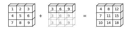
How about b -> (3, 1)?
In this case, NumPy will automatically expand b -> (3, 1) to b -> (3, 3).
Element-wise addition will then result in a matrix
b.shape = (3, 1)

a + b
array([[ 4, 5, 6],
[10, 11, 12],
[16, 17, 18]])Here is a visual representation of this broadcasting operation:
Source
fig = plt.figure(figsize=(5, 1), facecolor='w')
ax = plt.axes([0, 0, 1, 1], xticks=[], yticks=[], frameon=False)

# first block
draw_cube(ax, (1, 7.5), 1, depth, [1, 2, 3, 4, 5, 6, 9], '1', **solid)
draw_cube(ax, (2, 7.5), 1, depth, [1, 2, 3, 6, 9], '2', **solid)
draw_cube(ax, (3, 7.5), 1, depth, [1, 2, 3, 6, 7, 9, 10], '3', **solid)

draw_cube(ax, (1, 6.5), 1, depth, [2, 3, 4], '4', **solid)
draw_cube(ax, (2, 6.5), 1, depth, [2, 3], '5', **solid)
draw_cube(ax, (3, 6.5), 1, depth, [2, 3, 7, 10], '6', **solid)

draw_cube(ax, (1, 5.5), 1, depth, [2, 3, 4], '7', **solid)
draw_cube(ax, (2, 5.5), 1, depth, [2, 3], '8', **solid)
draw_cube(ax, (3, 5.5), 1, depth, [2, 3, 7, 10], '9', **solid)

# second block
draw_cube(ax, (6, 7.5), 1, depth, [1, 2, 3, 4, 5, 6, 7, 9, 10], '3', **solid)
draw_cube(ax, (7, 7.5), 1, depth, [1, 2, 3, 6, 7, 9, 10], '3', **dotted)
draw_cube(ax, (8, 7.5), 1, depth, [1, 2, 3, 6, 7, 9, 10], '3', **dotted)

draw_cube(ax, (6, 6.5), 1, depth, [2, 3, 4, 7, 10], '6', **solid)
draw_cube(ax, (7, 6.5), 1, depth, [2, 3, 6, 7, 9, 10, 11], '6', **dotted)
draw_cube(ax, (8, 6.5), 1, depth, [2, 3, 6, 7, 9, 10, 11], '6', **dotted)

draw_cube(ax, (6, 5.5), 1, depth, [2, 3, 4, 7, 10], '9', **solid)
draw_cube(ax, (7, 5.5), 1, depth, [2, 3, 7, 10, 11], '9', **dotted)
draw_cube(ax, (8, 5.5), 1, depth, [2, 3, 7, 10, 11], '9', **dotted)

# third block
draw_cube(ax, (12, 7.5), 1, depth, [1, 2, 3, 4, 5, 6, 9], '4', **solid)
draw_cube(ax, (13, 7.5), 1, depth, [1, 2, 3, 6, 9], '5', **solid)
draw_cube(ax, (14, 7.5), 1, depth, [1, 2, 3, 6, 7, 9, 10], '6', **solid)

draw_cube(ax, (12, 6.5), 1, depth, [2, 3, 4], '10', **solid)
draw_cube(ax, (13, 6.5), 1, depth, [2, 3], '11', **solid)
draw_cube(ax, (14, 6.5), 1, depth, [2, 3, 7, 10], '12', **solid)

draw_cube(ax, (12, 5.5), 1, depth, [2, 3, 4], '16', **solid)
draw_cube(ax, (13, 5.5), 1, depth, [2, 3], '17', **solid)
draw_cube(ax, (14, 5.5), 1, depth, [2, 3, 7, 10], '18', **solid)

ax.text(5, 7.0, '+', size=12, ha='center', va='center')
ax.text(10.5, 7.0, '=', size=12, ha='center', va='center');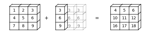
The previous broadcasting operation is equivalent to the following for loop
row, column = a.shape
result = np.empty((3, 3))
for i in range(row):
    for j in range(column):
        result[i, j] = a[i, j] + b[i,0]

result
array([[ 4., 5., 6.],
[10., 11., 12.],
[16., 17., 18.]])In some cases, both operands will be expanded.
When we have a -> (3,) and b -> (3, 1), a will be expanded to a -> (3, 3), and b will be expanded to b -> (3, 3).
In this case, element-wise addition will result in a matrix
a = np.array([3, 6, 9])
b = np.array([2, 3, 4])
b.shape = (3, 1)

a + b
array([[ 5, 8, 11],
[ 6, 9, 12],
[ 7, 10, 13]])Here is a visual representation of this broadcasting operation:
Source
# Draw a figure and axis with no boundary
fig = plt.figure(figsize=(5, 1), facecolor='w')
ax = plt.axes([0, 0, 1, 1], xticks=[], yticks=[], frameon=False)

# first block
draw_cube(ax, (1, 7.5), 1, depth, [1, 2, 3, 4, 5, 6, 9], '3', **solid)
draw_cube(ax, (2, 7.5), 1, depth, [1, 2, 3, 6, 9], '6', **solid)
draw_cube(ax, (3, 7.5), 1, depth, [1, 2, 3, 6, 7, 9, 10], '9', **solid)

draw_cube(ax, (1, 6.5), 1, depth, range(2, 13), '3', **dotted)
draw_cube(ax, (2, 6.5), 1, depth, [2, 3, 6, 7, 9, 10, 11], '6', **dotted)
draw_cube(ax, (3, 6.5), 1, depth, [2, 3, 6, 7, 9, 10, 11], '9', **dotted)

draw_cube(ax, (1, 5.5), 1, depth, [2, 3, 4, 7, 8, 10, 11, 12], '3', **dotted)
draw_cube(ax, (2, 5.5), 1, depth, [2, 3, 7, 10, 11], '6', **dotted)
draw_cube(ax, (3, 5.5), 1, depth, [2, 3, 7, 10, 11], '9', **dotted)

# second block
draw_cube(ax, (6, 7.5), 1, depth, [1, 2, 3, 4, 5, 6, 7, 9, 10], '2', **solid)
draw_cube(ax, (7, 7.5), 1, depth, [1, 2, 3, 6, 7, 9, 10], '2', **dotted)
draw_cube(ax, (8, 7.5), 1, depth, [1, 2, 3, 6, 7, 9, 10], '2', **dotted)

draw_cube(ax, (6, 6.5), 1, depth, [2, 3, 4, 7, 10], '3', **solid)
draw_cube(ax, (7, 6.5), 1, depth, [2, 3, 6, 7, 9, 10, 11], '3', **dotted)
draw_cube(ax, (8, 6.5), 1, depth, [2, 3, 6, 7, 9, 10, 11], '3', **dotted)

draw_cube(ax, (6, 5.5), 1, depth, [2, 3, 4, 7, 10], '4', **solid)
draw_cube(ax, (7, 5.5), 1, depth, [2, 3, 7, 10, 11], '4', **dotted)
draw_cube(ax, (8, 5.5), 1, depth, [2, 3, 7, 10, 11], '4', **dotted)

# third block
draw_cube(ax, (12, 7.5), 1, depth, [1, 2, 3, 4, 5, 6, 9], '5', **solid)
draw_cube(ax, (13, 7.5), 1, depth, [1, 2, 3, 6, 9], '8', **solid)
draw_cube(ax, (14, 7.5), 1, depth, [1, 2, 3, 6, 7, 9, 10], '11', **solid)

draw_cube(ax, (12, 6.5), 1, depth, [2, 3, 4], '6', **solid)
draw_cube(ax, (13, 6.5), 1, depth, [2, 3], '9', **solid)
draw_cube(ax, (14, 6.5), 1, depth, [2, 3, 7, 10], '12', **solid)

draw_cube(ax, (12, 5.5), 1, depth, [2, 3, 4], '7', **solid)
draw_cube(ax, (13, 5.5), 1, depth, [2, 3], '10', **solid)
draw_cube(ax, (14, 5.5), 1, depth, [2, 3, 7, 10], '13', **solid)

ax.text(5, 7.0, '+', size=12, ha='center', va='center')
ax.text(10.5, 7.0, '=', size=12, ha='center', va='center');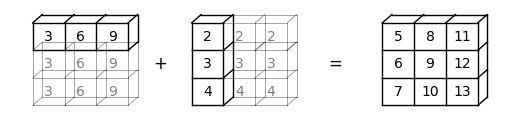
While broadcasting is very useful, it can sometimes seem confusing.
For example, let’s try adding a -> (3, 2) and b -> (3,).
a = np.array(
      [[1, 2],
       [4, 5],
       [7, 8]])
b = np.array([3, 6, 9])

a + b
---------------------------------------------------------------------------
ValueError Traceback (most recent call last)
Cell In[69], line 7
1 a = np.array(
2 [[1, 2],
3 [4, 5],
4 [7, 8]])
5 b = np.array([3, 6, 9])
----> 7 a + b
ValueError: operands could not be broadcast together with shapes (3,2) (3,) The ValueError tells us that operands could not be broadcast together.
Here is a visual representation to show why this broadcasting cannot be executed:
Source
# Draw a figure and axis with no boundary
fig = plt.figure(figsize=(3, 1.3), facecolor='w')
ax = plt.axes([0, 0, 1, 1], xticks=[], yticks=[], frameon=False)

# first block
draw_cube(ax, (1, 7.5), 1, depth, [1, 2, 3, 4, 5, 6, 9], '1', **solid)
draw_cube(ax, (2, 7.5), 1, depth, [1, 2, 3, 6, 7, 9, 10], '2', **solid)

draw_cube(ax, (1, 6.5), 1, depth, [2, 3, 4], '4', **solid)
draw_cube(ax, (2, 6.5), 1, depth, [2, 3, 7, 10], '5', **solid)

draw_cube(ax, (1, 5.5), 1, depth, [2, 3, 4], '7', **solid)
draw_cube(ax, (2, 5.5), 1, depth, [2, 3, 7, 10], '8', **solid)

# second block
draw_cube(ax, (6, 7.5), 1, depth, [1, 2, 3, 4, 5, 6, 9], '3', **solid)
draw_cube(ax, (7, 7.5), 1, depth, [1, 2, 3, 6, 9], '6', **solid)
draw_cube(ax, (8, 7.5), 1, depth, [1, 2, 3, 6, 7, 9, 10], '9', **solid)

draw_cube(ax, (6, 6.5), 1, depth, range(2, 13), '3', **dotted)
draw_cube(ax, (7, 6.5), 1, depth, [2, 3, 6, 7, 9, 10, 11], '6', **dotted)
draw_cube(ax, (8, 6.5), 1, depth, [2, 3, 6, 7, 9, 10, 11], '9', **dotted)

draw_cube(ax, (6, 5.5), 1, depth, [2, 3, 4, 7, 8, 10, 11, 12], '3', **dotted)
draw_cube(ax, (7, 5.5), 1, depth, [2, 3, 7, 10, 11], '6', **dotted)
draw_cube(ax, (8, 5.5), 1, depth, [2, 3, 7, 10, 11], '9', **dotted)


ax.text(4.5, 7.0, '+', size=12, ha='center', va='center')
ax.text(10, 7.0, '=', size=12, ha='center', va='center')
ax.text(11, 7.0, '?', size=16, ha='center', va='center');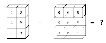
We can see that NumPy cannot expand the arrays to the same size.
It is because, when b is expanded from b -> (3,) to b -> (3, 3), NumPy cannot match b with a -> (3, 2).
Things get even trickier when we move to higher dimensions.
To help us, we can use the following list of rules:
Step 1: When the dimensions of two arrays do not match, NumPy will expand the one with fewer dimensions by adding dimension(s) on the left of the existing dimensions.
- For example, if
a -> (3, 3)andb -> (3,), then broadcasting will add a dimension to the left so thatb -> (1, 3); - If
a -> (2, 2, 2)andb -> (2, 2), then broadcasting will add a dimension to the left so thatb -> (1, 2, 2); - If
a -> (3, 2, 2)andb -> (2,), then broadcasting will add two dimensions to the left so thatb -> (1, 1, 2)(you can also see this process as going through Step 1 twice).
- For example, if
Step 2: When the two arrays have the same dimension but different shapes, NumPy will try to expand dimensions where the shape index is 1.
- For example, if
a -> (1, 3)andb -> (3, 1), then broadcasting will expand dimensions with shape 1 in bothaandbso thata -> (3, 3)andb -> (3, 3); - If
a -> (2, 2, 2)andb -> (1, 2, 2), then broadcasting will expand the first dimension ofbso thatb -> (2, 2, 2); - If
a -> (3, 2, 2)andb -> (1, 1, 2), then broadcasting will expandbon all dimensions with shape 1 so thatb -> (3, 2, 2).
- For example, if
Here are code examples for broadcasting higher dimensional arrays
# a -> (2, 2, 2) and  b -> (1, 2, 2)

a = np.array(
    [[[1, 2],
      [2, 3]],

     [[2, 3],
      [3, 4]]])
print(f'the shape of array a is {a.shape}')

b = np.array(
    [[1,7],
     [7,1]])
print(f'the shape of array b is {b.shape}')

a + b
the shape of array a is (2, 2, 2)
the shape of array b is (2, 2)
array([[[ 2,  9],
        [ 9,  4]],

       [[ 3, 10],
        [10,  5]]])
# a -> (3, 2, 2) and b -> (2,)
a = np.array(
[[[1, 2],
[3, 4]],
[[4, 5],
[6, 7]],
[[7, 8],
[9, 10]]])
print(f'the shape of array a is {a.shape}')
b = np.array([3, 6])
print(f'the shape of array b is {b.shape}')
a + bthe shape of array a is (3, 2, 2)
the shape of array b is (2,)
array([[[ 4,  8],
        [ 6, 10]],

       [[ 7, 11],
        [ 9, 13]],

       [[10, 14],
[12, 16]]])- Step 3: After Step 1 and 2, if the two arrays still do not match, a
ValueErrorwill be raised. For example, supposea -> (2, 2, 3)andb -> (2, 2)- By Step 1,
bwill be expanded tob -> (1, 2, 2); - By Step 2,
bwill be expanded tob -> (2, 2, 2); - We can see that they do not match each other after the first two steps. Thus, a
ValueErrorwill be raised
- By Step 1,
a = np.array(
    [[[1, 2, 3],
      [2, 3, 4]],

     [[2, 3, 4],
      [3, 4, 5]]])
print(f'the shape of array a is {a.shape}')

b = np.array(
    [[1,7],
     [7,1]])
print(f'the shape of array b is {b.shape}')

a + b
the shape of array a is (2, 2, 3)
the shape of array b is (2, 2)
---------------------------------------------------------------------------
ValueError                                Traceback (most recent call last)
Cell In[73], line 14
      9 b = np.array(
     10     [[1,7],
     11      [7,1]])
     12 print(f'the shape of array b is {b.shape}')
---> 14 a + b

ValueError: operands could not be broadcast together with shapes (2,2,3) (2,2) 11.6Mutability and Copying Arrays
NumPy arrays are mutable data types, like Python lists.
In other words, their contents can be altered (mutated) in memory after initialization.
We already saw examples above.
Here’s another example:
a = np.array([42, 44])
a
array([42, 44])a[-1] = 0 # Change last element to 0
aarray([42, 0])Mutability leads to the following behavior (which can be shocking to MATLAB programmers...)
a = np.random.randn(3)
a
array([-1.36503874, 0.52843985, -0.27011958])b = a
b[0] = 0.0
aarray([ 0. , 0.52843985, -0.27011958])What’s happened is that we have changed a by changing b.
The name b is bound to a and becomes just another reference to the
array the Python assignment model is described in more detail later in the course.
Hence, it has equal rights to make changes to that array.
This is in fact the most sensible default behavior!
It means that we pass around only pointers to data, rather than making copies.
Making copies is expensive in terms of both speed and memory.
11.6.1Making Copies
It is of course possible to make b an independent copy of a when required.
This can be done using np.copy
a = np.random.randn(3)
a
array([ 1.05041645, -1.54372669, -0.39072903])b = np.copy(a)
barray([ 1.05041645, -1.54372669, -0.39072903])Now b is an independent copy (called a deep copy)
b[:] = 1
b
array([1., 1., 1.])aarray([ 1.05041645, -1.54372669, -0.39072903])Note that the change to b has not affected a.
11.7Additional Functionality
Let’s look at some other useful things we can do with NumPy.
11.7.1Vectorized Functions
NumPy provides versions of the standard functions log, exp, sin, etc. that act element-wise on arrays
z = np.array([1, 2, 3])
np.sin(z)
array([0.84147098, 0.90929743, 0.14112001])This eliminates the need for explicit element-by-element loops such as
n = len(z)
y = np.empty(n)
for i in range(n):
    y[i] = np.sin(z[i])
Because they act element-wise on arrays, these functions are called vectorized functions.
In NumPy-speak, they are also called ufuncs, which stands for “universal functions”.
As we saw above, the usual arithmetic operations (+, *, etc.) also
work element-wise, and combining these with the ufuncs gives a very large set of fast element-wise functions.
zarray([1, 2, 3])(1 / np.sqrt(2 * np.pi)) * np.exp(- 0.5 * z**2)array([0.24197072, 0.05399097, 0.00443185])Not all user-defined functions will act element-wise.
For example, passing the function f defined below a NumPy array causes a ValueError
def f(x):
    return 1 if x > 0 else 0
The NumPy function np.where provides a vectorized alternative:
x = np.random.randn(4)
x
array([ 1.00515063, 0.20323953, 0.12391472, -0.85060523])np.where(x > 0, 1, 0) # Insert 1 if x > 0 true, otherwise 0array([1, 1, 1, 0])You can also use np.vectorize to vectorize a given function
f = np.vectorize(f)
f(x)                # Passing the same vector x as in the previous example
array([1, 1, 1, 0])However, this approach doesn’t always obtain the same speed as a more carefully crafted vectorized function.
11.7.2Comparisons
As a rule, comparisons on arrays are done element-wise
z = np.array([2, 3])
y = np.array([2, 3])
z == y
array([ True, True])y[0] = 5
z == yarray([False, True])z != yarray([ True, False])The situation is similar for >, <, >= and <=.
We can also do comparisons against scalars
z = np.linspace(0, 10, 5)
z
array([ 0. , 2.5, 5. , 7.5, 10. ])z > 3array([False, False, True, True, True])This is particularly useful for conditional extraction
b = z > 3
b
array([False, False, True, True, True])z[b]array([ 5. , 7.5, 10. ])Of course we can---and frequently do---perform this in one step
z[z > 3]array([ 5. , 7.5, 10. ])11.7.3Sub-packages
NumPy provides some additional functionality related to scientific programming through its sub-packages.
We’ve already seen how we can generate random variables using np.random
z = np.random.randn(10000)  # Generate standard normals
y = np.random.binomial(10, 0.5, size=1000)    # 1,000 draws from Bin(10, 0.5)
y.mean()np.float64(5.097)Another commonly used subpackage is np.linalg
A = np.array([[1, 2], [3, 4]])

np.linalg.det(A) # Compute the determinantnp.float64(-2.0000000000000004)np.linalg.inv(A) # Compute the inversearray([[-2. , 1. ],
[ 1.5, -0.5]])Much of this functionality is also available in SciPy, a collection of modules that are built on top of NumPy.
We’ll cover the SciPy versions in more detail soon.
For a comprehensive list of what’s available in NumPy see this documentation.
11.8Speed Comparisons
We mentioned in an previous lecture that NumPy-based vectorization can accelerate scientific applications.
In this section we try some speed comparisons to illustrate this fact.
11.8.1Vectorization vs Loops
Let’s begin with some non-vectorized code, which uses a native Python loop to generate, square and then sum a large number of random variables:
n = 1_000_000%%time
y = 0 # Will accumulate and store sum
for i in range(n):
x = random.uniform(0, 1)
y += x**2CPU times: user 608 ms, sys: 830 μs, total: 609 ms
Wall time: 1.58 s
The following vectorized code achieves the same thing.
%%time

x = np.random.uniform(0, 1, n)
y = np.sum(x**2)
CPU times: user 15 ms, sys: 2 ms, total: 17 ms
Wall time: 51.8 ms
As you can see, the second code block runs much faster. Why?
The second code block breaks the loop down into three basic operations
- draw
nuniforms - square them
- sum them
These are sent as batch operators to optimized machine code.
Apart from minor overheads associated with sending data back and forth, the result is C or Fortran-like speed.
When we run batch operations on arrays like this, we say that the code is vectorized.
The next section illustrates this point.
11.8.2Universal Functions
As discussed above, many functions provided by NumPy are universal functions (ufuncs).
By exploiting ufuncs, many operations can be vectorized, leading to faster execution.
For example, consider the problem of maximizing a function of two variables over the square .
For and let’s choose
Here’s a plot of
def f(x, y):
    return np.cos(x**2 + y**2) / (1 + x**2 + y**2)

xgrid = np.linspace(-3, 3, 50)
ygrid = xgrid
x, y = np.meshgrid(xgrid, ygrid)

fig = plt.figure(figsize=(10, 8))
ax = fig.add_subplot(111, projection='3d')
ax.plot_surface(x,
                y,
                f(x, y),
                rstride=2, cstride=2,
                cmap=cm.jet,
                alpha=0.7,
                linewidth=0.25)
ax.set_zlim(-0.5, 1.0)
ax.set_xlabel('$x$', fontsize=14)
ax.set_ylabel('$y$', fontsize=14)
plt.show()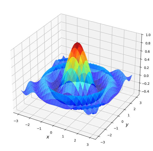
To maximize it, we’re going to use a naive grid search:
- Evaluate for all in a grid on the square.
- Return the maximum of observed values.
The grid will be
grid = np.linspace(-3, 3, 1000)Here’s a non-vectorized version that uses Python loops.
%%time

m = -np.inf

for x in grid:
    for y in grid:
        z = f(x, y)
        if z > m:
            m = z
CPU times: user 2.86 s, sys: 0 ns, total: 2.86 s
Wall time: 6.79 s
And here’s a vectorized version
%%time

x, y = np.meshgrid(grid, grid)
np.max(f(x, y))
CPU times: user 18.6 ms, sys: 17.9 ms, total: 36.5 ms
Wall time: 71.4 ms
np.float64(0.9999819641085747)In the vectorized version, all the looping takes place in compiled code.
As you can see, the second version is much faster.
11.9Exercises
Solution to Exercise 1
This code does the job
def p(x, coef):
    X = np.ones_like(coef)
    X[1:] = x
    y = np.cumprod(X)   # y = [1, x, x**2,...]
    return coef @ y
Let’s test it
x = 2
coef = np.linspace(2, 4, 3)
print(coef)
print(p(x, coef))
# For comparison
q = np.poly1d(np.flip(coef))
print(q(x))
[2. 3. 4.]
24.0
24.0
Solution to Exercise 2
Here’s our first pass at a solution:
from numpy import cumsum
from numpy.random import uniform

class DiscreteRV:
    """
    Generates an array of draws from a discrete random variable with vector of
    probabilities given by q.
    """

    def __init__(self, q):
        """
        The argument q is a NumPy array, or array like, nonnegative and sums
        to 1
        """
        self.q = q
        self.Q = cumsum(q)

    def draw(self, k=1):
        """
        Returns k draws from q. For each such draw, the value i is returned
        with probability q[i].
        """
        return self.Q.searchsorted(uniform(0, 1, size=k))
The logic is not obvious, but if you take your time and read it slowly, you will understand.
There is a problem here, however.
Suppose that q is altered after an instance of discreteRV is
created, for example by
q = (0.1, 0.9)
d = DiscreteRV(q)
d.q = (0.5, 0.5)
The problem is that Q does not change accordingly, and Q is the
data used in the draw method.
To deal with this, one option is to compute Q every time the draw
method is called.
But this is inefficient relative to computing Q once-off.
A better option is to use descriptors.
A solution from the quantecon library using descriptors that behaves as we desire can be found here.
Solution to Exercise 3
An example solution is given below.
In essence, we’ve just taken this code from QuantEcon and added in a plot method
"""
Modifies ecdf.py from QuantEcon to add in a plot method

"""

class ECDF:
    """
    One-dimensional empirical distribution function given a vector of
    observations.

    Parameters
    ----------
    observations : array_like
        An array of observations

    Attributes
    ----------
    observations : array_like
        An array of observations

    """

    def __init__(self, observations):
        self.observations = np.asarray(observations)

    def __call__(self, x):
        """
        Evaluates the ecdf at x

        Parameters
        ----------
        x : scalar(float)
            The x at which the ecdf is evaluated

        Returns
        -------
        scalar(float)
            Fraction of the sample less than x

        """
        return np.mean(self.observations <= x)

    def plot(self, ax, a=None, b=None):
        """
        Plot the ecdf on the interval [a, b].

        Parameters
        ----------
        a : scalar(float), optional(default=None)
            Lower endpoint of the plot interval
        b : scalar(float), optional(default=None)
            Upper endpoint of the plot interval

        """

        # === choose reasonable interval if [a, b] not specified === #
        if a is None:
            a = self.observations.min() - self.observations.std()
        if b is None:
            b = self.observations.max() + self.observations.std()

        # === generate plot === #
        x_vals = np.linspace(a, b, num=100)
        f = np.vectorize(self.__call__)
        ax.plot(x_vals, f(x_vals))
        plt.show()
Here’s an example of usage
fig, ax = plt.subplots()
X = np.random.randn(1000)
F = ECDF(X)
F.plot(ax)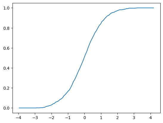
Solution to Exercise 4
Part 1 Solution
np.random.seed(123)
x = np.random.randn(4, 4)
y = np.random.randn(4)
C = np.empty_like(x)
n = len(x)
for i in range(n):
for j in range(n):
C[i, j] = x[i, j] / y[j]Compare the results to check your answer
print(C)Output
[[-0.49214189  0.45607819  0.28183596 -3.90043439]
 [-0.26229311  0.75518888 -2.41688145 -1.11063629]
 [ 0.57387869 -0.39635354 -0.67614513 -0.2452416 ]
 [ 0.676082   -0.29216483 -0.44218937 -1.12471925]]
You can also use array_equal() to check your answer
print(np.array_equal(A, C))True
Part 2 Solution
np.random.seed(123)
x = np.random.randn(1000, 100, 100)
y = np.random.randn(100)
qe.tic()
D = np.empty_like(x)
d1, d2, d3 = x.shape
for i in range(d1):
for j in range(d2):
for k in range(d3):
D[i, j, k] = x[i, j, k] / y[k]
qe.toc()TOC: Elapsed: 0:00:12.46
12.462379455566406Note that the for loop takes much longer than the broadcasting operation.
Compare the results to check your answer
print(D)Output
[[[ 1.85764005 -0.89419976  0.24485371 ... -3.04214618  0.17711597
   -0.22643801]
  [-1.09863014  1.77333433  0.61630351 ... -0.24732757 -0.15931155
   -0.13015397]
  [-1.20344529  0.53624915  1.90420857 ...  0.92748804  0.07494711
    0.48954772]
  ...
  [-1.09763323  0.68632802 -1.21568707 ... -3.87025031 -0.19456046
    0.18331773]
  [-0.47546852 -0.16883695  2.92991418 ... -0.05967182 -0.20796073
   -0.49082994]
  [ 1.14380091  1.93460538 -0.76305492 ... -1.0537099   0.27167901
    0.57963424]]

 [[ 2.12344323  0.28058176 -0.73457091 ...  3.55049699  0.59737154
   -0.31414907]
  [ 1.40074417 -0.09113173  0.50276294 ... -1.85572391  0.13914077
   -0.93776321]
  [ 2.35739042 -0.79089649  0.20835615 ... -0.11001198  0.86250367
   -1.26949634]
  ...
  [ 2.11831946  0.15242396 -0.17269536 ...  0.03469371 -0.06074779
    0.10114045]
  [-0.08300138  0.47232405 -0.89930099 ...  0.66104947 -0.45183377
   -1.05885526]
  [ 0.282155   -1.44848315 -1.25832989 ... -3.12998376  0.48762406
    0.22052869]]

 [[-1.76517625 -1.19419485  0.08293115 ...  0.7919151  -0.03812759
   -1.19540255]
  [-0.66639955  0.16580616 -0.32083535 ...  0.72351825 -0.72239583
   -0.46386281]
  [-0.45163238 -1.5262587  -0.38541194 ...  1.82015759  0.23151272
    0.81609303]
  ...
  [ 1.14317214 -0.60571044 -0.74962613 ... -3.13330221  0.61817627
    0.37738869]
  [-0.65686356  0.41024983  0.2700362  ... -0.08588743  0.20408508
    0.33667429]
  [-0.43851304  0.58339651 -0.9076869  ... -2.55408527 -0.22112928
    0.9912754 ]]

 ...

 [[ 1.13470002 -0.20836287 -0.50483798 ...  0.32733859 -0.32203002
    0.43385307]
  [-0.11763272 -0.77698937 -0.46659376 ...  2.01256989 -0.19222608
   -0.48021737]
  [ 0.89558661  0.93447059  0.35386499 ... -1.2218747   0.42826019
    0.73980809]
  ...
  [-0.30040698 -1.14758822 -1.2785068  ...  3.9600491  -0.25830068
   -1.09906439]
  [-2.89569174 -0.67988752 -0.26342148 ...  0.62855881  0.05570693
   -0.05084807]
  [ 0.87738281 -2.37555322  1.66177996 ...  0.09857952  0.35564132
   -1.22140972]]

 [[-3.31843223  0.19402721  0.87502303 ... -1.47591384 -0.25236749
   -0.85281481]
  [-2.84794867 -0.31042414  0.43040259 ... -4.01127498  0.06267678
   -0.2073196 ]
  [-0.47909317 -0.77256923 -0.49818879 ... -0.17526151  0.64720631
   -0.06831215]
  ...
  [ 0.35509683 -0.48189502 -0.18528007 ...  2.03614189 -0.15287291
    0.0979404 ]
  [-1.20730244 -0.24269721 -0.28048927 ...  0.94378219 -0.21283324
   -0.30738091]
  [-1.81004008  1.01260185 -0.62311067 ... -0.03158149 -0.36355966
    0.43427753]]

 [[-1.43227284 -0.20319046  1.37271425 ...  2.34113161  0.18025411
   -0.247025  ]
  [ 0.47792311  0.61186236  0.73460309 ... -1.52671835 -0.10967386
   -0.04788996]
  [-1.51873339  0.73425213 -0.54033092 ...  0.21434631 -0.31597544
   -0.24364054]
  ...
  [-0.24128379 -0.72604109 -0.36722827 ...  2.20219708  1.04943754
   -0.44221604]
  [-1.43364744  0.54701702  1.08795598 ...  0.19549939 -0.12604844
   -0.74936097]
  [-0.59335595  0.46807169 -0.04178975 ... -1.1783837   0.0395992
    0.55109001]]]
print(np.array_equal(B, D))True

Creative Commons License – This work is licensed under a Creative Commons Attribution-ShareAlike 4.0 International.